37. Multilayer Perceptrons
Multilayer perceptrons
Implementing the hidden layer
Prerequisites
Below, we are going to walk through the math of neural networks in a multilayer perceptron. With multiple perceptrons, we are going to move to using vectors and matrices. To brush up, be sure to view the following:
- Khan Academy's introduction to vectors .
- Khan Academy's introduction to matrices .
Derivation
Before, we were dealing with only one output node which made the code straightforward. However now that we have multiple input units and multiple hidden units, the weights between them will require two indices: w_{ij} where i denotes input units and j are the hidden units.
For example, the following image shows our network, with its input units labeled x_1, x_2, and x_3 , and its hidden nodes labeled h_1 and h_2 :
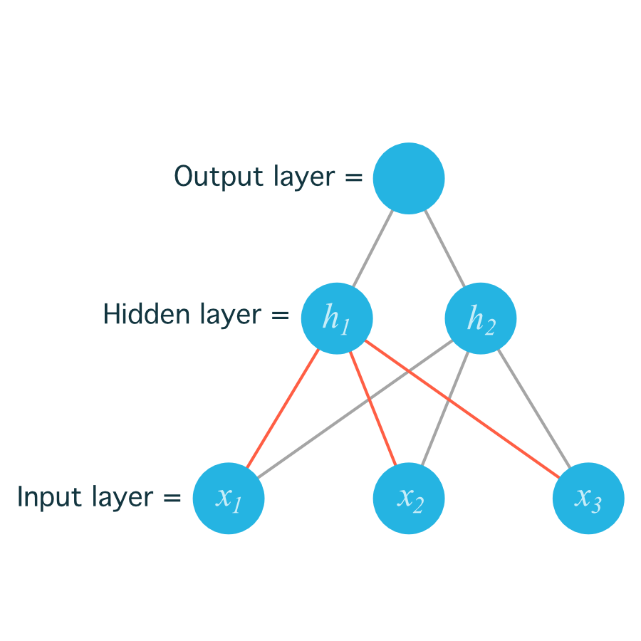
The lines indicating the weights leading to h_1 have been colored differently from those leading to h_2 just to make it easier to read.
Now to index the weights, we take the input unit number for the _i and the hidden unit number for the _j . That gives us
w_{11}
for the weight leading from x_1 to h_1 , and
w_{12}
for the weight leading from x_1 to h_2 .
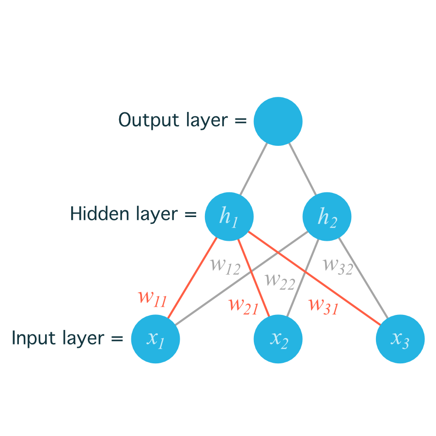
The following image includes all of the weights between the input layer and the hidden layer, labeled with their appropriate w_{ij} indices:
Before, we were able to write the weights as an array, indexed as w_i .
But now, the weights need to be stored in a matrix , indexed as w_{ij} . Each row in the matrix will correspond to the weights leading out of a single input unit , and each column will correspond to the weights leading in to a single hidden unit . For our three input units and two hidden units, the weights matrix looks like this:
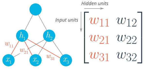
Be sure to compare the matrix above with the diagram shown before it so you can see where the different weights in the network end up in the matrix.
To initialize these weights in Numpy, we have to provide the shape of the matrix. If
features
is a 2D array containing the input data:
# Number of records and input units
n_records, n_inputs = features.shape
# Number of hidden units
n_hidden = 2
weights_input_to_hidden = np.random.normal(0, n_inputs**-0.5, size=(n_inputs, n_hidden))
This creates a 2D array (i.e. a matrix) named
weights_input_to_hidden
with dimensions
n_inputs
by
n_hidden
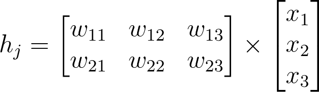
. Remember how the input to a hidden unit is the sum of all the inputs multiplied by the hidden unit's weights. So for each hidden layer unit,
h_j
, we need to calculate the following:

To do that, we now need to use matrix multiplication .
In this case, we're multiplying the inputs (a row vector here) by the weights. To do this, you take the dot (inner) product of the inputs with each column in the weights matrix. For example, to calculate the input to the first hidden unit, j = 1 , you'd take the dot product of the inputs with the first column of the weights matrix, like so:
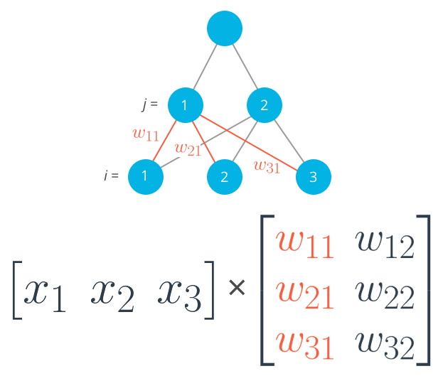
Calculating the input to the first hidden unit with the first column of the weights matrix.

And for the second hidden layer input, you calculate the dot product of the inputs with the second column. And so on and so forth.
In NumPy, you can do this for all the inputs and all the outputs at once using
np.dot
hidden_inputs = np.dot(inputs, weights_input_to_hidden)
You could also define your weights matrix such that it has dimensions
n_hidden
by
n_inputs
then multiply like so where the inputs form a
column vector
:
Note: The weight indices have changed in the above image and no longer match up with the labels used in the earlier diagrams. That's because, in matrix notation, the row index always precedes the column index, so it would be misleading to label them the way we did in the neural net diagram. Just keep in mind that this is the same weight matrix as before, but rotated so the first column is now the first row, and the second column is now the second row. If we were to use the labels from the earlier diagram, the weights would fit into the matrix in the following locations:
Weight matrix shown with labels matching earlier diagrams.
Remember, the above is not a correct view of the indices , but it uses the labels from the earlier neural net diagrams to show you where each weight ends up in the matrix.
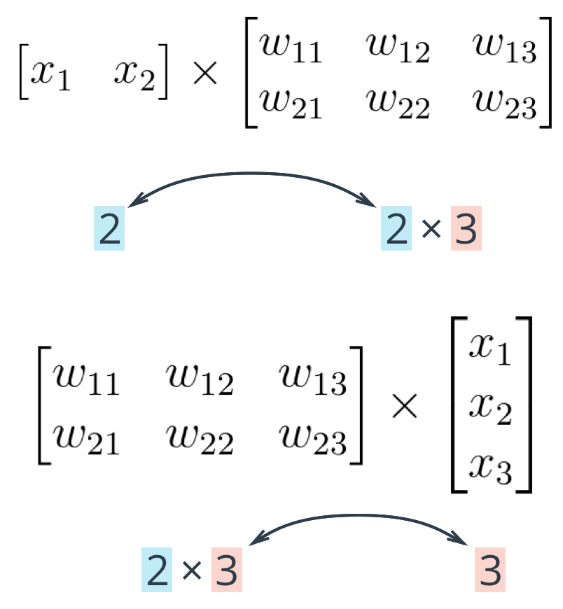
The important thing with matrix multiplication is that the dimensions match . For matrix multiplication to work, there has to be the same number of elements in the dot products. In the first example, there are three columns in the input vector, and three rows in the weights matrix. In the second example, there are three columns in the weights matrix and three rows in the input vector. If the dimensions don't match, you'll get this:
# Same weights and features as above, but swapped the order
hidden_inputs = np.dot(weights_input_to_hidden, features)
---------------------------------------------------------------------------
ValueError                                Traceback (most recent call last)
<ipython-input-11-1bfa0f615c45> in <module>()
----> 1 hidden_in = np.dot(weights_input_to_hidden, X)

ValueError: shapes (3,2) and (3,) not aligned: 2 (dim 1) != 3 (dim 0)
The dot product can't be computed for a 3x2 matrix and 3-element array. That's because the 2 columns in the matrix don't match the number of elements in the array. Some of the dimensions that could work would be the following:
The rule is that if you're multiplying an array from the left, the array must have the same number of elements as there are rows in the matrix. And if you're multiplying the matrix from the left, the number of columns in the matrix must equal the number of elements in the array on the right.
Making a column vector
You see above that sometimes you'll want a column vector, even though by default Numpy arrays work like row vectors. It's possible to get the transpose of an array like so
arr.T
, but for a 1D array, the transpose will return a row vector. Instead, use
arr[:,None]
to create a column vector:
print(features)
> array([ 0.49671415, -0.1382643 ,  0.64768854])

print(features.T)
> array([ 0.49671415, -0.1382643 ,  0.64768854])

print(features[:, None])
> array([[ 0.49671415],
       [-0.1382643 ],
       [ 0.64768854]])
Alternatively, you can create arrays with two dimensions. Then, you can use
arr.T
to get the column vector.
np.array(features, ndmin=2)
> array([[ 0.49671415, -0.1382643 ,  0.64768854]])

np.array(features, ndmin=2).T
> array([[ 0.49671415],
       [-0.1382643 ],
       [ 0.64768854]])
I personally prefer keeping all vectors as 1D arrays, it just works better in my head.
Programming quiz
Below, you'll implement a forward pass through a 4x3x2 network, with sigmoid activation functions for both layers.
Things to do:
- Calculate the input to the hidden layer.
- Calculate the hidden layer output.
- Calculate the input to the output layer.
- Calculate the output of the network.
Start Quiz: